验证曲线validation_curve

validation_curve()的作用

误差是由偏差（bias）、方差（variance）、噪声（noise）组成。 偏差：模型对于不同的训练样本集，预测结果的平均误差 方差：模型对于不同训练样本集的敏感程度 噪声：数据集本身的一项属性 同样的数据，（cos函数上的点加上噪声），我们用同样的模型（polynomial），但是超参数却不同（degree =1,4,15）,会得到不同的拟合效果：

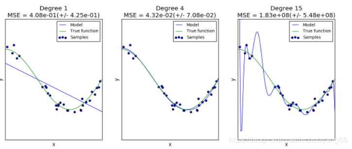
第一个模型太简单，模型本身就拟合不了这些数据（高偏差，underfitting）； 第二个模型可以看成几乎完美地拟合了数据； 第三个模型完美拟合了几乎所有的训练数据，但却不能很好的拟合真实的函数，也就是对于不同的训练数据很敏感（高方差，overfitting）。 对于以上第一和第三个模型，我们可以选择模型和超参数来得到效果更好的配置，也就是可以通过验证曲线（validation_curve）来调节。

validation_curve的含义

证曲线（validation_curve）和学习曲线（sklearn.model_selection.learning_curve()）的区别是，验证曲线的横轴为某个超参数，如一些树形集成学习算法中的max_depth、min_sample_leaf等等。 从验证曲线上可以看到随着超参数设置的改变，模型可能从欠拟合到合适，再到过拟合的过程，进而选择一个合适的位置，来提高模型的性能。 需要注意的是，如果我们使用验证分数来优化超参数，那么该验证分数是有偏差的，它无法再代表魔心的泛化能力，我们就需要使用其他测试集来重新评估模型的泛化能力。 即一般我们需要把一个数据集分成三部分：train、validation和test，我们使用train训练模型，并通过在 validation数据集上的表现不断修改超参数值（例如svm中的C值，gamma值等），当模型超参数在validation数据集上表现最优时，我们再使用全新的测试集test进行测试，以此来衡量模型的泛化能力。

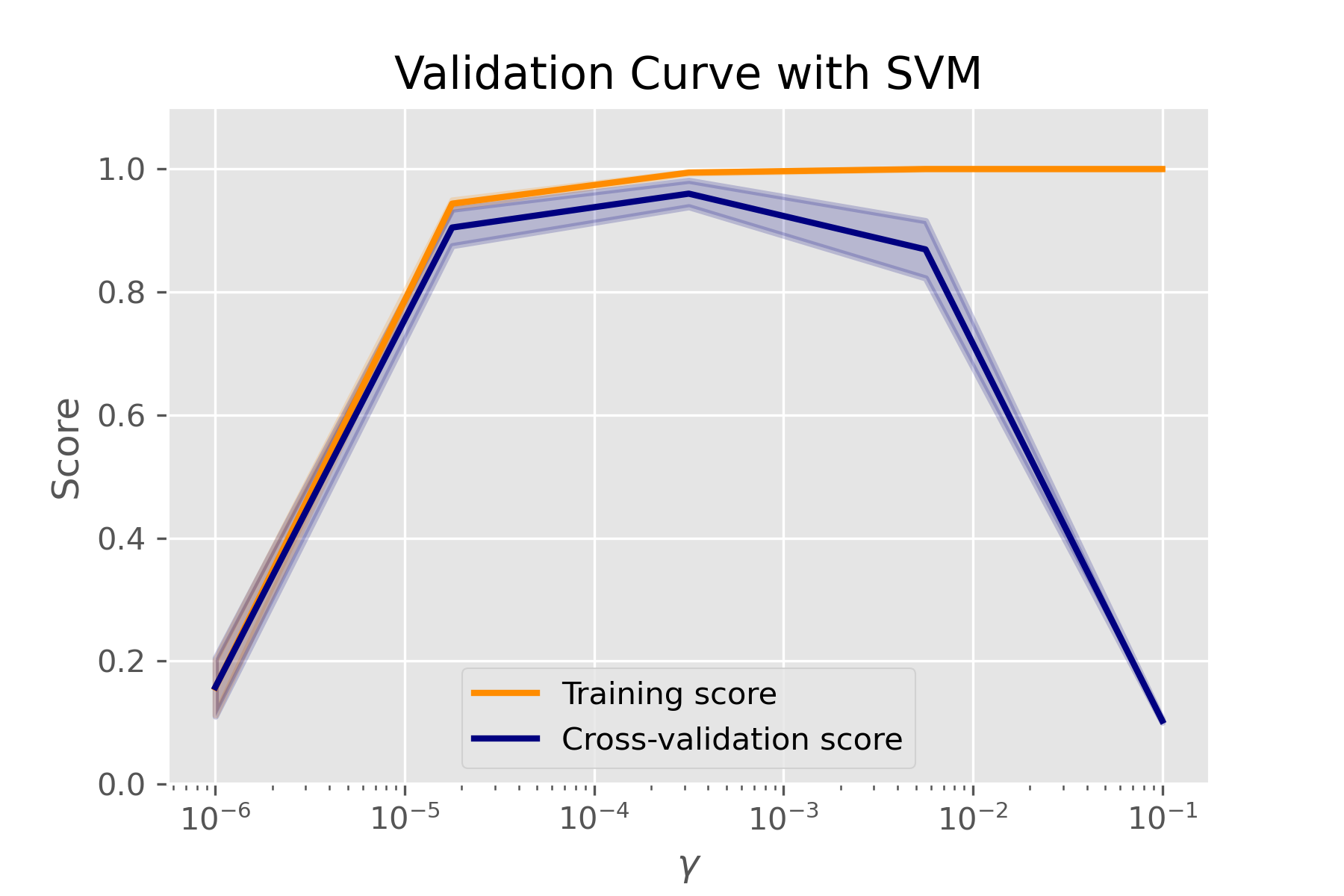
不过有时画出单个超参数与训练分数和验证分数的关系图，有助于观察该模型在该超参数取值时，是否过拟合或欠拟合的情况发生，如下两个图：

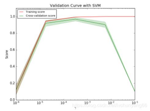
如图是SVM在不同gamma时，它在训练集和交叉验证上的分数： gamma很小时，训练分数和验证分数都很低，为欠拟合； gamma逐渐增加时，两个分数都较高，此时模型相对不错； gamma太高时，训练分数高，验证分数低，学习器会过拟合。 本例中，可以选验证集准确率开始下降，而测试集越来越高那个转折点作为gamma的最优选择。

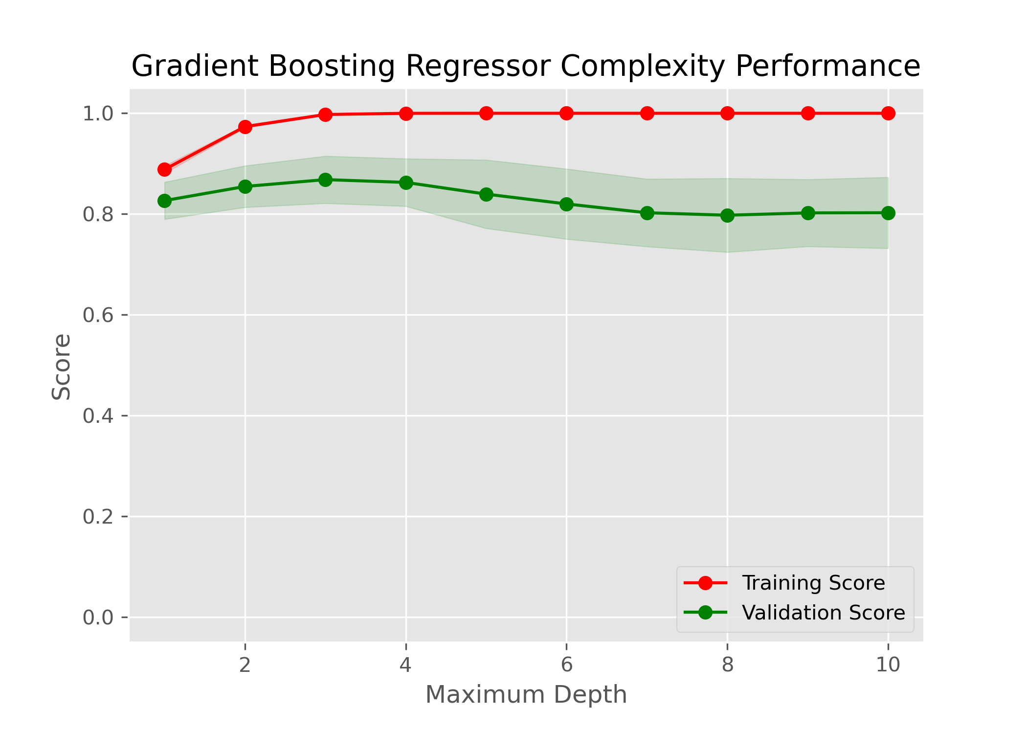
如上图，max_depth的最佳值应该定位5

函数

validation_curve 是展示某个因子，不同取值的算法得分

sklearn.model_selection.validation_curve(estimator, 
                                         X, y, *, 
                                         param_name, 
                                         param_range, 
                                         groups=None, 
                                         cv=None, 
                                         scoring=None, 
                                         n_jobs=None, 
                                         pre_dispatch='all', 
                                         verbose=0, 
                                         error_score=nan)

参数

• estimator : 评估器

• X : 训练集

• y： 训练集对应的标签

• param_name : str ,要改变的参数的名字，如果当model为SVC时，改变gamma的值，求最好的那个gamma值

• param_rang: array-like of shape (n_values,) 给定的参数范围

• cv : 交叉验证生成器或可迭代的，可选的 确定交叉验证拆分策略。cv的可能输入是：

  • None，要使用默认的 5 折交叉验证
  • int, to specify the number of folds in a (Stratified)KFold,
  • CV splitter,
  • An iterable yielding (train, test) splits as arrays of indices.

  For int/None inputs, if the estimator is a classifier and y is either binary or multiclass, StratifiedKFold is used. In all other cases, KFold is used.

• scoring: str or callable, default=Non 打分类型，如 accuracy ,r2 等，

返回值：

• train_scores ：array of shape (n_ticks, n_cv_folds)

• Scores on training sets.

• est_scores：array of shape (n_ticks, n_cv_folds) Scores on test set.

案例 1

import matplotlib.pyplot as plt
import numpy as np

from sklearn.datasets import load_digits
from sklearn.svm import SVC
from sklearn.model_selection import validation_curve

X, y = load_digits(return_X_y=True)

param_range = np.logspace(-6, -1, 5)
train_scores, test_scores = validation_curve(
    SVC(), X, y, param_name="gamma", param_range=param_range,
    scoring="accuracy", n_jobs=1)

train_scores_mean = np.mean(train_scores, axis=1)
train_scores_std = np.std(train_scores, axis=1)
test_scores_mean = np.mean(test_scores, axis=1)
test_scores_std = np.std(test_scores, axis=1)

plt.title("Validation Curve with SVM")
plt.xlabel(r"$\gamma$")
plt.ylabel("Score")
plt.ylim(0.0, 1.1)
lw = 2
plt.semilogx(param_range, train_scores_mean, label="Training score",
             color="darkorange", lw=lw)
plt.fill_between(param_range, train_scores_mean - train_scores_std,
                 train_scores_mean + train_scores_std, alpha=0.2,
                 color="darkorange", lw=lw)
plt.semilogx(param_range, test_scores_mean, label="Cross-validation score",
             color="navy", lw=lw)
plt.fill_between(param_range, test_scores_mean - test_scores_std,
                 test_scores_mean + test_scores_std, alpha=0.2,
                 color="navy", lw=lw)
plt.legend(loc="best")

案例 2

带有 cv 参数

import numpy as np
import pandas as pd
from time import time
import matplotlib.pyplot as plt
from sklearn.ensemble import GradientBoostingRegressor
from sklearn.model_selection import ShuffleSplit
from sklearn.model_selection import validation_curve


def ModelComplexity(X, y):
    """ Calculates the performance of the model as model complexity increases.
        The learning and testing errors rates are then plotted. """

    # Create 10 cross-validation sets for training and testing
    cv = ShuffleSplit(n_splits=10, test_size=0.2, random_state=0)

    # Vary the max_depth parameter from 1 to 10
    max_depth = np.arange(1, 11)
    start = time()

    # Calculate the training and testing scores
    train_scores, test_scores = validation_curve(GradientBoostingRegressor(), X, y,
                                                 param_name="max_depth", 
                                                 param_range=max_depth, 
                                                 cv=cv, 
                                                 scoring='r2')

    print(time()-start)

    # Find the mean and standard deviation for smoothing
    train_mean = np.mean(train_scores, axis=1)
    train_std = np.std(train_scores, axis=1)
    test_mean = np.mean(test_scores, axis=1)
    test_std = np.std(test_scores, axis=1)

    # Plot the validation curve
    plt.figure(figsize=(7, 5))
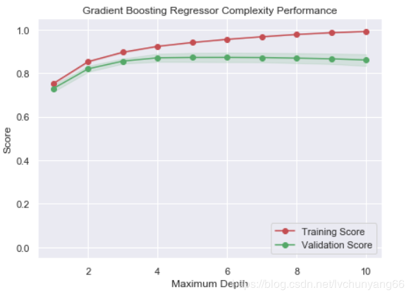
    plt.title('Gradient Boosting Regressor Complexity Performance')
    plt.plot(max_depth, train_mean, 'o-', color='r', label='Training Score')
    plt.plot(max_depth, test_mean, 'o-', color='g', label='Validation Score')
    plt.fill_between(max_depth, train_mean - train_std,
                     train_mean + train_std, alpha=0.15, color='r')
    plt.fill_between(max_depth, test_mean - test_std,
                     test_mean + test_std, alpha=0.15, color='g')

    # Visual aesthetics
    plt.legend(loc='lower right')
    plt.xlabel('Maximum Depth')
    plt.ylabel('Score')
    plt.ylim([-0.05, 1.05])



ModelComplexity(X_train, y_train)

画图时，横轴为 param_range，纵轴为 scoreing：

参考

• sklearn.model_selection.validation_curve
• validation_curve验证曲线与超参数