拟合curve_fit
scipy.optimize 中有 curve_fit方法可以拟合自定义的曲线,如指数函数拟合,幂指函数拟合和多项式拟合
scipy.optimize.curve_fit(f,
                         xdata,
                         ydata,
                         p0=None,
                         sigma=None, absolute_sigma=False,
                         check_finite=True, bounds=- inf,
                         inf, method=None, jac=None, **kwargs)
参数:
f模型函数f(x,…)。它必须将自变量作为第一个参数,并将要拟合的参数作为单独的剩余参数。xdata: array_like or object, 要拟合的自变量数组ydata: array_like, 要拟合的因变量的值p0:初始迭代值sigma:y值的不确定性的度量absolute_sigma: If False, sigma denotes relative weights of the data points. The returned covariance matrix pcov is based on estimated errors in the data, and is not affected by the overall magnitude of the values in sigma. Only the relative magnitudes of the sigma values matter.If True, sigma describes one standard deviation errors of the input data points. The estimated covariance in pcov is based on these values.check_finite:如果为True,则检测输入中是否有nan或者infbounds:指定变量的取值范围method:指定求解算法。可以为'lm'/'trf'/'dogbox'kwargs:传递给leastsq/least_squares的关键字参数。
返回值:
popt:最优化参数pcov:The estimated covariance of popt.
基本使用
用样本拟合函数
import numpy as np
import matplotlib.pyplot as plt
from scipy.optimize import curve_fit
# 定义目标函数
def func(x, a, b, c):
return a*np.exp(-b*x)+c
# 这部分生成样本点,对函数值加上高斯噪声作为样本点
# [0, 4]共50个点
xdata = np.linspace(0, 4, 50)
#
# a=2.5, b=1.3, c=0.5
y = func(xdata, 2.5, 1.3, 0.5)
np.random.seed(1)
err_stdev = 0.2
# 生成均值为0,标准差为err_stdev为0.2的高斯噪声
y_noise = err_stdev*np.random.normal(size=len(xdata))
ydata = y + y_noise
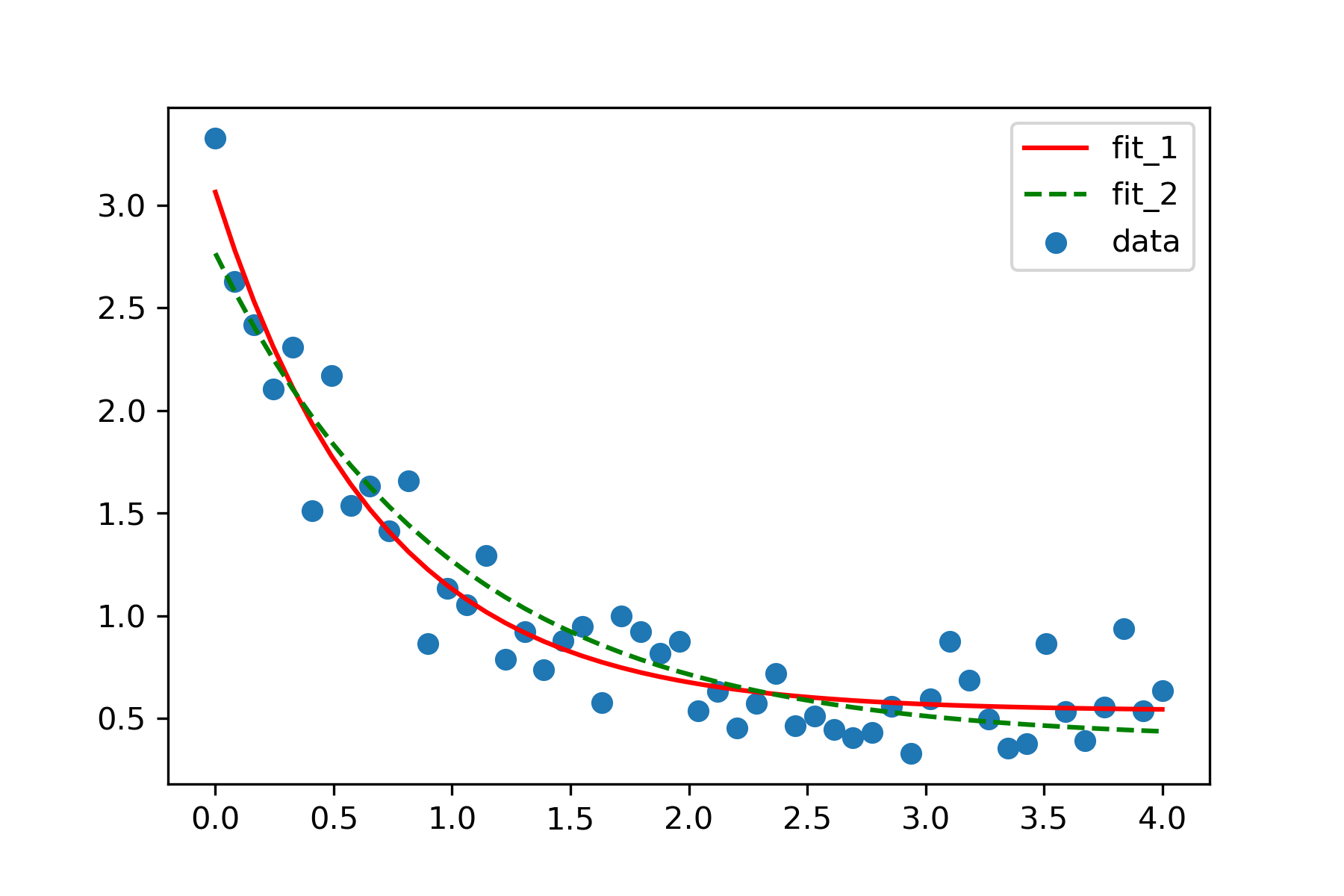
plt.scatter(xdata, ydata, label='data')
# 利用curve_fit作简单的拟合,popt为拟合得到的参数,pcov是参数的协方差矩阵
popt_1, pcov = curve_fit(func, xdata, ydata)
print(popt_1) #[2.52560138 1.44826091 0.53725085]
plt.plot(xdata, func(xdata, *popt_1), 'r-', label='fit_1')
# 限定参数范围:0<=a<=3, 0<=b<=1, 0<=c<=0.5
popt_2, pcov = curve_fit(func, xdata, ydata, bounds=(0, [3., 1., 0.5]))
print(popt_2) # [2.37032282 1. 0.39448271]
plt.plot(xdata, func(xdata, *popt_2), 'g--', label='fit_2')
plt.legend()
计算拟合结果的指标
总平方和 $SST$:
总平方和(SST) = 回归平方和(SSR)十残差平方和(SSE)
回归平方和 $SSR$ :
残差平方和 $SSE$ :
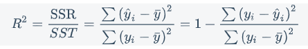
判定系数:
$MSE$ (均方差、方差):
$RMSE$(均方根、标准差):
def get_indexes(y_predict, y_data):
    n = y_data.size

    #计算 残差平方方差 SSE
    SSE = ((y_data - y_predict)**2).sum()

    # 均方差 MSE
    MSE = SSE / n

    # 均方根 RMSE 越接近 0,拟合效果越好
    RMSE = np.sqrt(MSE)

    # 求R方,0<=R<=1,越靠近1,拟合效果越好
    u = y_data.mean()
    SST = ((y_data - u)**2).sum()
    SSR = SST - SSE
    R_square = SSR / SST

    return SSE, MSE, RMSE, R_square
比较上一节的两次拟合,哪个拟合得更好
# 比较上一节的两次拟合,哪个拟合得更好
y_predict_1=func(xdata, *popt_1)
indexes_1=get_indexes(y_predict_1, ydata)
print(indexes_1)


# 模型2
y_predict_2=func(xdata, *popt_2)
indexes_2=get_indexes(y_predict_2, ydata)
print(indexes_2)
结果:
(1.833619516810147, 0.03667239033620294, 0.19150036641271195, 0.9163487663138368)
(2.306216123348346, 0.04612432246696692, 0.21476573857803047, 0.8947885195939563)