一维插值interp1d
interp1d类进行一维插值
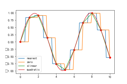
一维数据的插值运算可以通过函数interp1d()完成。
interp1d(x, y, kind='linear', ...)
其中,x和y参数是一系列已知的数据点,kind参数是插值类型,可以是字符串或整数,它给出插值的B样条曲线的阶数,候选值及作用下表所示:
| 候选值 | 作用 |
|---|---|
| ‘zero’ 、'nearest' | 阶梯插值,相当于0阶B样条曲线 |
| ‘slinear’ 、'linear' | 线性插值,用一条直线连接所有的取样点,相当于一阶B样条曲线 |
| ‘quadratic’ 、'cubic' | 二阶和三阶B样条曲线,更高阶的曲线可以直接使用整数值指定 |
interp1d比Matlab的interp有些优势,因为返回的是函数,不需要在事先设定需要求解的点,而是在需要使用时调用函数。
import numpy as np
import pylab as pl
from scipy import interpolate

import matplotlib as mpl
mpl.rcParams['font.sans-serif'] = ['SimHei']

x = np.linspace(0,10,11)
y = np.sin(x)

xnew = np.linspace(0,10,101)
pl.plot(x,y,'ro')

for kind in ['nearest', 'zero', 'slinear', 'quadratic']:
    f = interpolate.interp1d(x,y,kind=kind)
    ynew = f(xnew)
    pl.plot(xnew, ynew,label=str(kind))
pl.legend()
UnivariateSpline
interp1d不能外推运算(外插值)UnivariateSpline可以外插值
class scipy.interpolate.UnivariateSpline(x, y,
                                         w=None,
                                         bbox=[None, None],
                                         k=3,
                                         s=None
                                        )
- x,y是X-Y坐标数组
- w是每个数据点的权重值
- k为样条曲线的阶数
- s为平滑参数。
- s=0,样条曲线强制通过所有数据点
- s>0,满足
s=0强制通过所有数据点的外插值
from scipy import interpolate
import numpy as np
x1=np.linspace(0,10,20)
y1=np.sin(x1)

sx1=np.linspace(0,12,100)
func1=interpolate.UnivariateSpline(x1,y1,s=0)#强制通过所有点
sy1=func1(sx1)

import matplotlib.pyplot as plt
plt.plot(x1,y1,'o')
plt.plot(sx1,sy1)
plt.show()
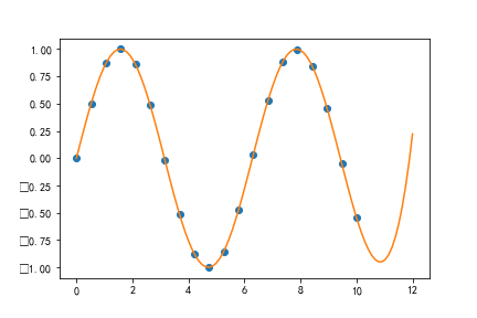
也就插值到(0,12),范围再大就不行了,毕竟插值的专长不在于预测
s>0:不强制通过所有点
import numpy as np
from scipy import interpolate
x2=np.linspace(0,20,200)
y2=np.sin(x2)+np.random.normal(loc=0,scale=1,size=len(x2))*0.2

sx2=np.linspace(0,22,2000)
func2=interpolate.UnivariateSpline(x2,y2,s=8)
sy2=func2(sx2)

import matplotlib.pyplot as plt
plt.plot(x2,y2,'.')
plt.plot(sx2,sy2)
plt.show()

__call__(x[, nu]) |
Evaluate spline (or its nu-th derivative) at positions x. |
|---|---|
antiderivative([n]) |
Construct a new spline representing the antiderivative of this spline. |
derivative([n]) |
Construct a new spline representing the derivative of this spline. |
derivatives(x) |
返回点 x 处样条曲线的导数。 |
get_coeffs() |
返回样条系数。 |
get_knots() |
Return positions of (boundary and interior) knots of the spline. |
get_residual() |
Return weighted sum of squared residuals of the spline approximation: sum((w[i] * (y[i]-s(x[i])))**2, axis=0). |
integral(a, b) |
返回两个给定点之间样条曲线的定积分。. |
roots() |
返回样条曲线的零点. |
set_smoothing_factor(s) |
Continue spline computation with the given smoothing factor s and with the knots found at the last call. |
print(np.array_str(func2.roots(), precision=3))
# [ 0.046  3.152  6.299  9.349 12.67  15.793 18.813]
参数插值
使用参数插值连接二维平面上的点
x = [
    4.913, 4.913, 4.918, 4.938, 4.955, 4.949, 4.911, 4.848, 4.864, 4.893,
    4.935, 4.981, 5.01, 5.021
]

y = [
    5.2785, 5.2875, 5.291, 5.289, 5.28, 5.26, 5.245, 5.245, 5.2615, 5.278,
    5.2775, 5.261, 5.245, 5.241
]

pl.plot(x, y, "o")

for s in (0, 1e-4):
    tck, t = interpolate.splprep([x, y], s=s)  #❶
    xi, yi = interpolate.splev(np.linspace(t[0], t[-1], 200), tck)  #❷
    pl.plot(xi, yi, lw=2, label=u"s=%g" % s)

pl.legend()

scipy.interpolate包里提供了两个函数splev和splrep共同完成(B-样条:贝兹曲线(又称贝塞尔曲线))插值,和之前一元插值一步就能完成不同,样条插值需要两步完成,第一步先用splrep计算出b样条曲线的参数tck,第二步在第一步的基础上用splev计算出各取样点的插值结果。
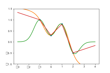
一元函数的 Rbf 插值
lass scipy.interpolate.Rbf(*args)
参数:
args:arrays
x, y, z, …, d, where x, y, z, … are the coordinates of the nodes and d is the array of values at the nodes
function:str or callable, optional 基于半径r的径向基函数,默认值为欧几里得距离; 默认值为“ multiquadric”
'multiquadric': sqrt((r/self.epsilon)**2 + 1)
'inverse': 1.0/sqrt((r/self.epsilon)**2 + 1)
'gaussian': exp(-(r/self.epsilon)**2)
'linear': r
'cubic': r**3
'quintic': r**5
'thin_plate': r**2 * log(r)
一维RBF插值
from scipy.interpolate import Rbf

x1 = np.array([-1, 0, 2.0, 1.0])
y1 = np.array([1.0, 0.3, -0.5, 0.8])

funcs = ['multiquadric', 'gaussian', 'linear']
nx = np.linspace(-3, 4, 100)
rbfs = [Rbf(x1, y1, function=fname) for fname in funcs]  #❶
rbf_ys = [rbf(nx) for rbf in rbfs]  #❷

pl.plot(x1, y1, "o")
for fname, ny in zip(funcs, rbf_ys):
    pl.plot(nx, ny, label=fname, lw=2)

pl.ylim(-1.0, 1.5)
pl.legend()
for fname, rbf in zip(funcs, rbfs):
    print (fname, rbf.nodes)

# multiquadric [-0.88822885  2.17654513  1.42877511 -2.67919021]
# gaussian [ 1.00321945 -0.02345964 -0.65441716  0.91375159]
# linear [-0.26666667  0.6         0.73333333 -0.9       ]