最小二乘法函数拟合leastsq

最小二乘估计原理是这样的： $y=f(x, \theta)+\varepsilon$ 其中 ε 独立同分布。 $\theta=\arg \min \sum\left(y_{i}-f\left(x_{i}, \theta\right)\right)^{2}$ 非线性最小二乘法中，SST=SSR+SSE不再成立，但仍然可以定义R_squared=1-SSE/SST

leastsq可以用来做最小二乘估计，可以在线性拟合和非线性拟合中使用。

leastsq

scipy.optimize.leastsq(func, 
                       x0, args=(), 
                       Dfun=None, full_output=0, 
                       col_deriv=0, ftol=1.49012e-08, 
                       xtol=1.49012e-08, gtol=0.0, 
                       maxfev=0, epsfcn=None, 
                       factor=100, diag=None)

参数：

一般我们只要指定前三个参数就可以了:

• func :是我们自己定义的一个计算误差的函数，
• x0 :是计算的初始参数值
• args：tuple, optional 是指定func的其他参数，都放在这个元组中

• func：是个可调用对象，给出每次拟合的残差。最开始的参数是待优化参数；后面的参数由args给出
• x0：初始迭代值
• args：一个元组，用于给func提供额外的参数。
• Dfun：用于计算func的雅可比矩阵（按行排列）。默认情况下，算法自动推算。它给出残差的梯度。最开始的参数是待优化参数；后面的参数由args给出
• full_output：如果非零，则给出更详细的输出
• col_deriv：如果非零，则计算雅可比矩阵更快（按列求导）
• ftol：指定相对的均方误差的阈值
• xtol：指定参数解收敛的阈值
• gtol：Orthogonality desired between the function vector and the columns of the Jacobian
• maxfev：设定算法迭代的最大次数。如果为零：如果为提供了Dfun，则为 100*(N+1)，N为x0的长度；如果未提供Dfun,则为200*(N+1)
• epsfcn：采用前向差分算法求解雅可比矩阵时的步长。
• factor：它决定了初始的步长
• diag：它给出了每个变量的缩放因子

返回值：

• x：拟合解组成的数组
• cov_x：Uses the fjac and ipvt optional outputs to construct an estimate of the jacobian around the solution
• infodict：给出了可选的输出。它是个字典，其中的键有：
  • nfev：func调用次数
  • fvec：最终的func输出
  • fjac：A permutation of the R matrix of a QR factorization of the final approximate Jacobian matrix, stored column wise.
  • ipvt：An integer array of length N which defines a permutation matrix, p, such that fjacp = qr, where r is upper triangular with diagonal elements of nonincreasing magnitude
• ier：一个整数标记。如果为 1/2/3/4，则表示拟合成功
• mesg：一个字符串。如果解未找到，则它给出详细信息

基本使用

线性拟合

import numpy as np
import matplotlib.pyplot as plt
from scipy.optimize import leastsq

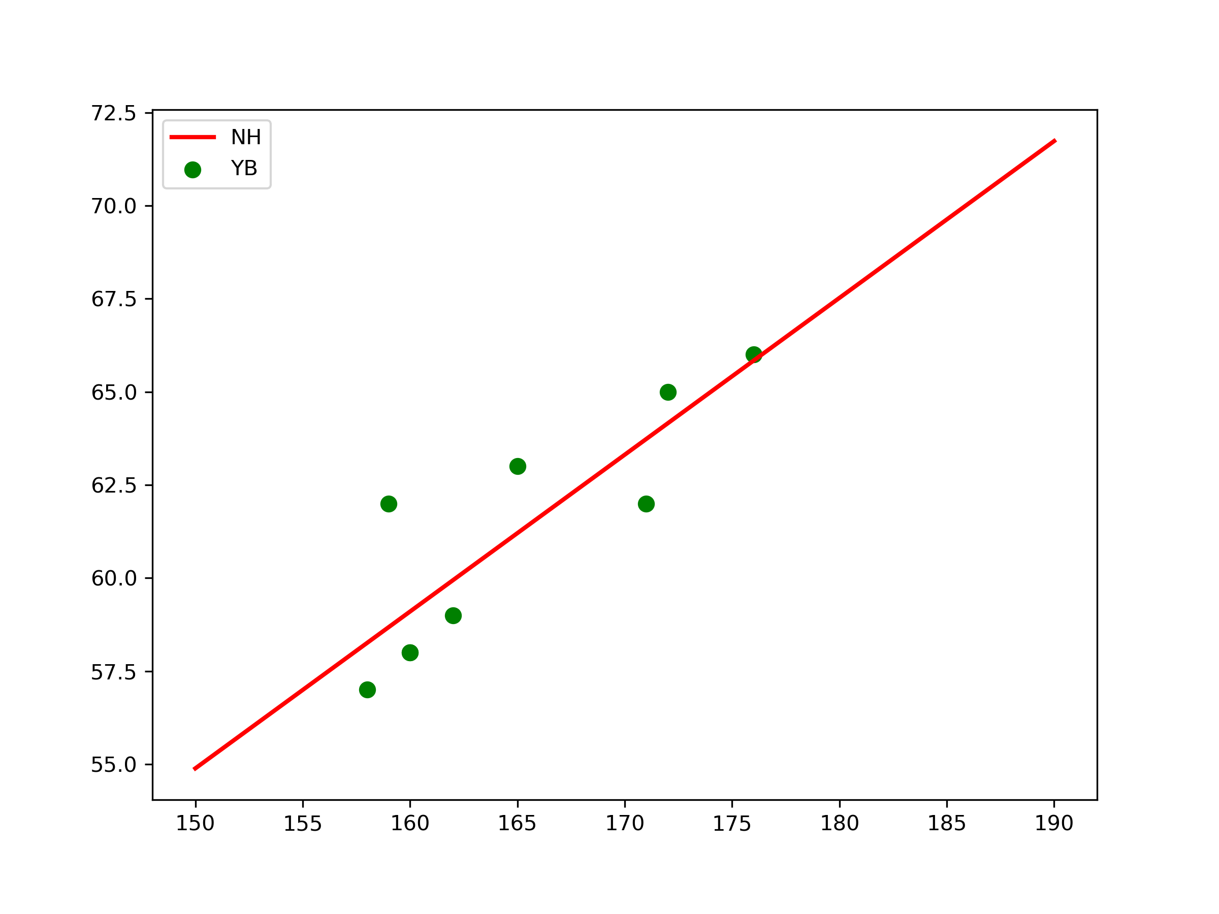
# 样本数据(Xi,Yi)，需要转换成数组(列表)形式
Xi = np.array([160, 165, 158, 172, 159, 176, 160, 162, 171])
Yi = np.array([58, 63, 57, 65, 62, 66, 58, 59, 62])

定义残差并寻优:

# 需要拟合的函数func :指定函数的形状 k= 0.42116973935 b= -8.28830260655
def func(p, x):
    k, b = p
    return k*x+b

# 偏差函数：x,y都是列表:这里的x,y更上面的Xi,Yi中是一一对应的
def error(p, x, y):
    return func(p, x)-y

给定初始值，进行拟合

# k,b的初始值，可以任意设定,经过几次试验，发现p0的值会影响cost的值：Para[1]
p0 = [1, 20]

# 把error函数中除了p0以外的参数打包到args中(使用要求)
Para = leastsq(error, p0, args=(Xi, Yi))

读取结果：

# 读取结果
k, b = Para[0]
print("k=", k, "b=", b)

计算误差:

残差平方和

def S(k,b):
    error=np.zeros(k.shape)
    for x,y in zip(X,Y):
        error+=(y-(k*x+b))**2
    return error
S(k,b)
# array(405808.61964307)

可视化：

# 画样本点
plt.figure(figsize=(8, 6))  # 指定图像比例： 8：6
plt.scatter(Xi, Yi, color="green", label="YB", linewidth=2)

# 画拟合直线
x = np.linspace(150, 190, 100)  # 在150-190直接画100个连续点
y = k*x+b  # 函数式
plt.plot(x, y, color="red", label="NH", linewidth=2)
plt.legend()  # 绘制图例

曲线拟合

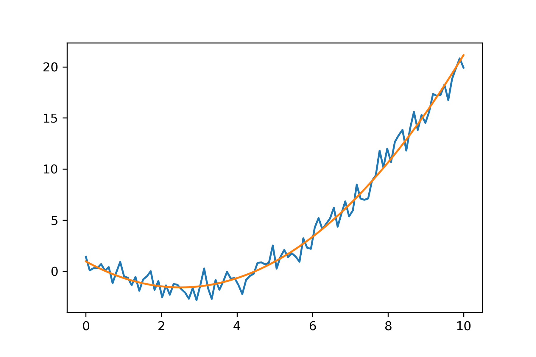
定义目标函数，准备一一检验其拟合效果

# 目标函数
def test_func(x, p):
    a, b, c = p
    return a*x**2+b*x+c

# 残差
def residuals(p,y,x):
    return y-test_func(x,p)

生成模拟数据

p_true = [0.4, -2, 0.9]  # 真实值

X = np.linspace(0, 10, 100)
y = test_func(X, p_true)+np.random.randn(len(X))

拟合

from scipy.optimize import leastsq


# 先验的估计，真实数据分析流程中，先预估一个接近的值。这里为了测试效果，先验设定为 1
p_prior = np.ones_like(p_true)

plsq = leastsq(residuals, p_prior, args=(y, X))

print(p_true)
print(plsq)

[0.4, -2, 0.9]
(array([ 0.40067724, -1.99507171,  0.86224339]), 3)

画图

import matplotlib.pyplot as plt
plt.plot(X, y)
plt.plot(X, test_func(X, plsq[0]))

参考

• cipy中最小二乘法函数leastsq的用法及其实例应用
• 【最小二乘估计】scipy.optimize.leastsq